Homework: Source separation
Use PCA, and multiple diagonalization to generate various projections of EEG data.
-
Load the file eeg-vep.mat from the class webpage. It should have epoched data with 160 channels, 545 samples and 116 trials saved in variable eeg.
-
Stack up the trials so that you have a data matrix of channels by samples (160 x 1630).
-
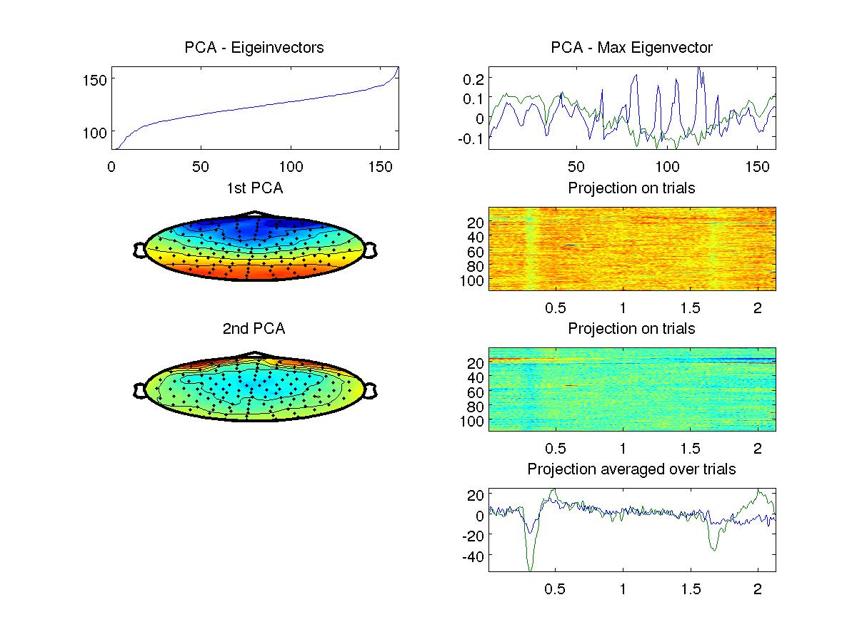
Compute the covariance and from this principal components of this data. Show the eigenvalue spectrum (on a dB scale. Note that this data has one zero eigenvalue due to "common mean subtraction". set the ylim such that you can see the relevant non-zero eigenvalues). Display first two principal component (the eigenvector with the strongest eigenvalue) on the scalp using the topoplot() function using the corresponding location file provided on the website. You will find that the first is negative in the front and positive in the back of the head. The second component with be positive around the eyes.
-
Project the data onto the first two principal component and display the result as images of trials by samples (116x545 for each of the two components). Also show the average across trials for the two components (two curves using plot).
This is how your figure might look like
Extra credit:
The follwing steps do not give particularly good results on this data, but you can implement them for extra credit if you like.
-
Repeat steps 2 trough 4 using instead the first and second half of the samples (samples 1:272 and 273:545) to obtain two covariance matrices. Find the eigenvectors that diagonalize both these matrices, e.g. generalized eigenvectors. Be sure to select the largets eigenvalues (see sample code below)
-
Repeat step 5 but now using the covariance of all the data and as the second correlation matrix use the the cross-correlation of the data with a version of the data that is delayed by K samples (try different delays). Be sure to symmetrize this matrix with Rxy=0.5*(Rxy+Rxy');
In total you should have 3 figures similar to the figure above with results for 3 different techniques (steps 4, 5 and 6). If you do not do the extra credit you will have just one figure. For each method combine plots with subplot into single figure. Label all axis and use milliseconds on the time axis.
Here some simple code to help you get started:
load eeg-vep.mat
[N,D,T]=size(eeg);

erp=squeeze(mean(eeg,1));
subplot(1,2,1); imagesc(time,1:D,squeeze(mean(eeg,1)));
ylabel('electrodes');xlabel('time (ms)')
subplot(1,2,2); topoplot(mean(erp(:,60:90),2),'BioSemi160.loc'); axis equal

% sample code to sort columns of eigenvectors U in ascending order
% of eigenvalues in diagonal matrix D.
[Y,I] = sort(diag(D));
U = U(:,I); D=diag(Y);